Outline
- DeepWalk: intro to graph embeddings
- DeepWalk example
- Node2Vec
- DeepGL
- References
Graph and graph embeddings
$$
G = (V, E, X, Y)
$$$$
f(X) \rightarrow Y
$$
- $V$: vertices
- $E$: edges
- $X$: attributes
- $Y$: labels
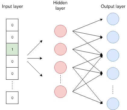
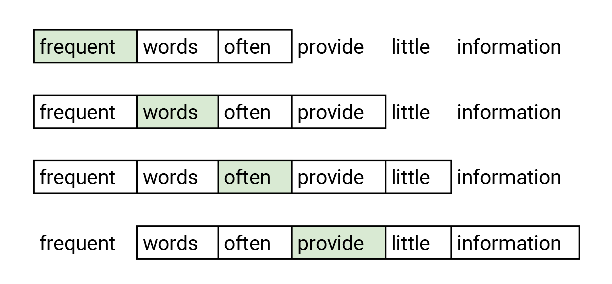
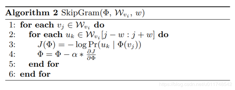
Word2Vec (SkipGram)
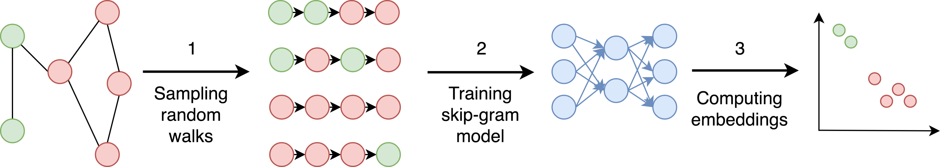
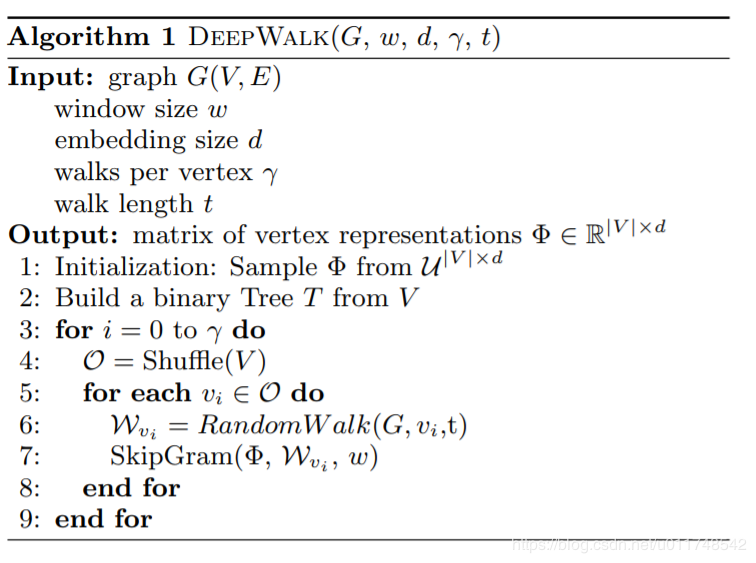
DeepWalk
From sentence embeddings to graph embeddings
In [2]:
import numpy as np
import networkx as nx
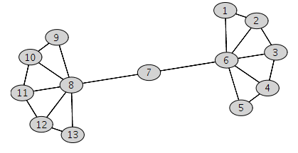
nx_graph = nx.Graph()
nodes = list(np.arange(1, 14))
# fmt: off
edges = [
(1, 2), (2, 3), (3, 4), (4, 5),
(1, 6), (2, 6), (3, 6), (4, 6), (5, 6),
(6, 7),
(7, 8),
(9, 8), (10, 8), (11, 8), (12, 8), (13, 8),
(9, 10), (10, 11), (11, 12), (12, 13),
]
# fmt: on
nx_graph.add_nodes_from(nodes)
nx_graph.add_edges_from(edges)
nx.draw(nx_graph, with_labels=True, node_color="white")

In [3]:
# https://github.com/phanein/deepwalk/blob/master/deepwalk/__main__.py
import random

import deepwalk
from deepwalk import walks as serialized_walks
from deepwalk.skipgram import Skipgram
from gensim.models import Word2Vec
from six import iterkeys
In [4]:
deepwalk_graph = deepwalk.graph.Graph()

for idx, x in enumerate(nx_graph.nodes()):
    for y in iterkeys(nx_graph[x]):
        deepwalk_graph[x].append(y)

deepwalk_graph.make_undirected()
deepwalk_graph
Out[4]:
In [5]:
# hyper-params

# num random walks per node: 80
NUM_WALKS = 80
# length of one random walk: 40
WALK_LENGTH = 40
# window size 10
WINDOW_SIZE = 10
# embedding dim 128
EMBEDDING_DIM = 128
In [6]:
walks = deepwalk.graph.build_deepwalk_corpus(
    deepwalk_graph,
    num_paths=NUM_WALKS,
    path_length=WALK_LENGTH,
    alpha=0,
    rand=random.Random(123)
)
print(np.array(walks))
print(np.array(walks).shape)
In [7]:
model = Word2Vec(
    walks,
    size=EMBEDDING_DIM,
    window=WINDOW_SIZE,
    min_count=0,
    sg=1,
    hs=1,
    workers=1,
)
In [8]:
# nodes, or "vocabulary"
model.wv.vocab
Out[8]:
In [9]:
# "word" embeddings
model.wv["1"]
Out[9]:
In [10]:
model.most_similar("1")
Out[10]:
In [11]:
nx.draw(nx_graph, with_labels=True, node_color="white")

In [12]:
# Visualisation of "word" embeddings using PCA
from sklearn.decomposition import PCA
from matplotlib import pyplot

def plot_pca(model):
    X = model[model.wv.vocab]
    pca = PCA(n_components=2)
    result = pca.fit_transform(X)

    pyplot.scatter(result[:, 0], result[:, 1])
    words = list(model.wv.vocab)
    for i, word in enumerate(words):
        pyplot.annotate(word, xy=(result[i, 0], result[i, 1]))
    pyplot.show()

plot_pca(model)

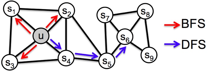
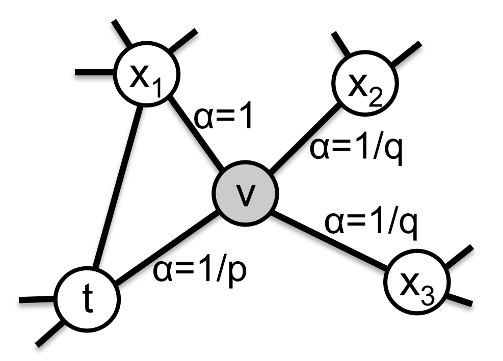
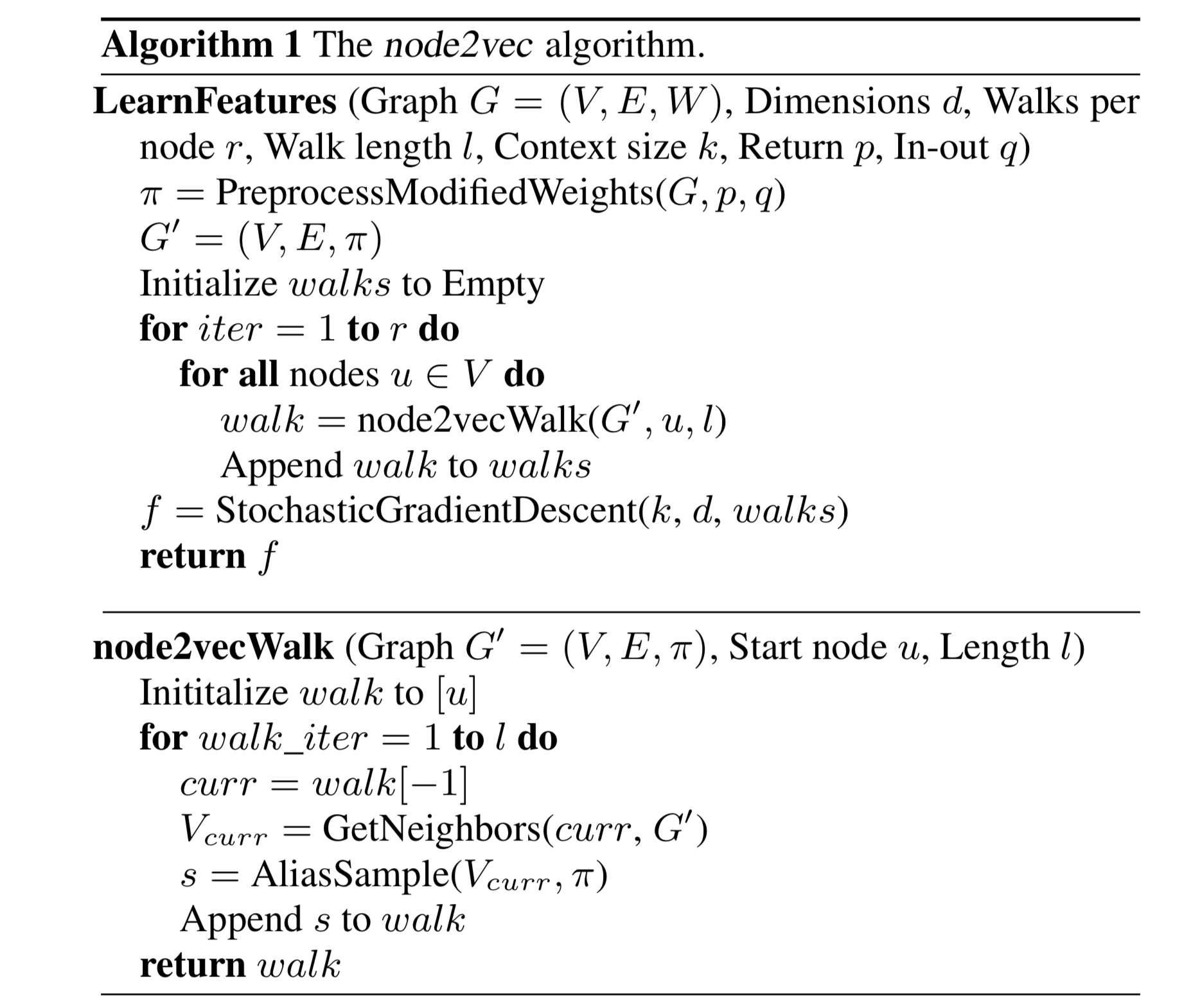
Node2Vec
Search strategies
- BFS: Breadth-first Sampling
- DFS: Depth-first Sampling
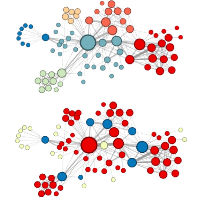
Node similarities in embedding space
- Homophily:
- Similarity in terms of the neighbouring of nodes
- Structural equivalence:
- Similarity in terms of structural roles; not emphasized on connectivity
2nd order random walk:
- Mixture of BFS and DFS
- Search bias $\alpha$:
- $p$: likelihood of immediately revisiting a node
- $q$: larger $q$ biased towards reversion, smaller $q$ biased towards visiting new nodes
- semi-supervised learning: decide p, q from labeled nodes
In [13]:
from node2vec import Node2Vec
In [14]:
node2vec = Node2Vec(
    nx_graph, dimensions=EMBEDDING_DIM, walk_length=WALK_LENGTH, num_walks=NUM_WALKS
)
In [15]:
print(
    "walks: \n", np.array(node2vec.walks),
    "\n\n",
    "shape: ", np.array(node2vec.walks).shape
)
In [16]:
model = node2vec.fit(window=WINDOW_SIZE, min_count=0)
In [17]:
model.wv.vocab
Out[17]:
In [18]:
plot_pca(model)

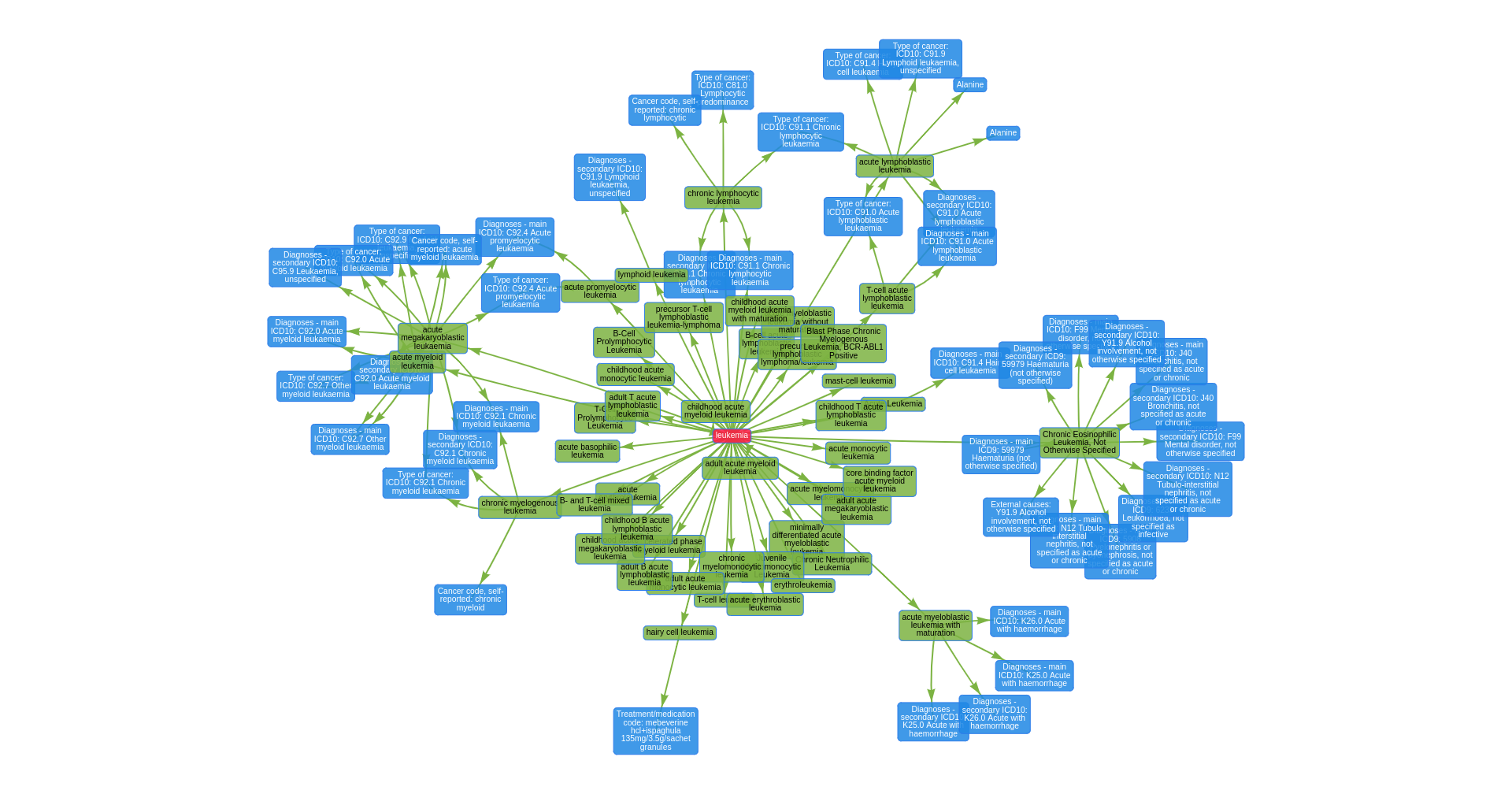
EpiGraphDB
In [19]:
import json

with open("assets/epigraphdb_efo_leukemia.json", "r") as f:
    epigraphdb_data = json.load(f)
In [20]:
from pprint import pprint
pprint(epigraphdb_data["nodes"][:3])
pprint(epigraphdb_data["edges"][:3])
In [21]:
epigraphdb_graph = nx.Graph()
epigraphdb_graph.add_nodes_from([item["id"] for item in epigraphdb_data["nodes"]])
epigraphdb_graph.add_edges_from([(item["from"], item["to"]) for item in epigraphdb_data["edges"]])
nx.draw(epigraphdb_graph, with_labels=True, node_color="white")

In [22]:
epigraphdb_node2vec = Node2Vec(
    epigraphdb_graph, dimensions=EMBEDDING_DIM, walk_length=WALK_LENGTH, num_walks=NUM_WALKS
)
In [23]:
epigraphdb_model = epigraphdb_node2vec.fit(window=WINDOW_SIZE, min_count=0)
In [24]:
plot_pca(epigraphdb_model)

In [25]:
epigraphdb_model.most_similar("24")
Out[25]:
In [26]:
from sklearn.manifold import TSNE

def plot_tsne(model):
    X = model[model.wv.vocab]
    result = TSNE(n_components=2).fit_transform(X)

    pyplot.scatter(result[:, 0], result[:, 1])
    words = list(model.wv.vocab)
    for i, word in enumerate(words):
        pyplot.annotate(word, xy=(result[i, 0], result[i, 1]))
    pyplot.show()

plot_tsne(epigraphdb_model)

References
- DeepWalk: https://arxiv.org/abs/1403.6652
- Node2Vec: https://cs.stanford.edu/~jure/pubs/node2vec-kdd16.pdf
- http://media.cs.tsinghua.edu.cn/~multimedia/cuipeng/papers/Network%20Representation-Tutorial.pdf
- https://medium.com/@_init_/an-illustrated-explanation-of-using-skipgram-to-encode-the-structure-of-a-graph-deepwalk-6220e304d71b
- https://towardsdatascience.com/graph-embeddings-the-summary-cc6075aba007
- https://towardsdatascience.com/node2vec-embeddings-for-graph-data-32a866340fef
- https://neo4j.com/online-summit/session/graph-embeddings-machine-learning-ml